The annual peak shaving project allows users to specify a new peak demand limit following project implementation and assumes that users do not already have information about the size of the energy storage project. Therefore, in addition to the project’s impacts, the energy storage system’s power and energy capacity are reported by the project module. For projects which the energy storage project's specifications are known, daily peak reduction may be a good alternative. In the annual peak shaving project, the sole objective of the system is to limit the annual peak demand to the prescribed demand limit.
The figure below provides a process flow diagram showing how the project module operates within the larger context of the tool.
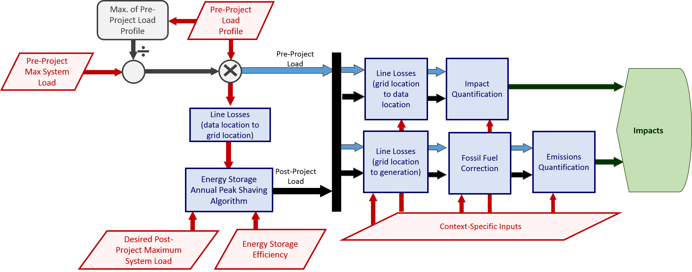
Algorithm Outputs
The annual peak shaving algorithm outputs a modified load profile as well as the calculated maximum charge/discharge rate, energy capacity, and final state of charge for the energy storage system (ESS). The modified load profiles can then be used to quantify other project impacts.
Algorithm Description
The ESS’s maximum charge and discharge rates are assumed to be equal and are calculated based on the power required to reduce the pre-project load to within the demand limit. In other words, the maximum ESS rate of discharge will be the difference between the original load profile’s peak value and the allowable post-project maximum demand as defined by users. The algorithm assumes that the ESS is fully charged at the beginning of the period. Each successive hour is then checked for violations of the demand limit. If an hourly load exceeds this value, the ESS is set to discharge sufficient energy during that hour to reduce load to this post-project maximum load value. As soon as load drops below the maximum, the ESS is set to recharge until full or until load again exceeds the demand limit and the ESS must again inject power to resolve the violation. The ESS will charge at its maximum charge rate or the maximum rate possible without causing load to exceed the post-project demand limit, whichever is less. No attempt is made to target times of low demand for ESS charging; recharging will occur as soon as feasible within the project’s constraints.
The ESS is called upon to serve load that exceeds the user-defined demand limit, and this dictates its requisite energy capacity. The first of such events will size the ESS so that it can exactly meet this excess load. When another event occurs, the ESS’s current available energy will be used. If the energy available is not sufficient to reduce load to within the limit, the size of the ESS is increased accordingly. The energy capacity of the ESS is therefore determined dynamically as the algorithm runs. If there is not sufficient time or available energy for the ESS to recharge before the end of the period without violating the demand limit, the ESS’s final state of charge will be less than 100%. The algorithm therefore reports the final state of charge in addition to the ESS’s power and energy capacities. It is left to the user’s discretion to determine whether the ESS’s inability to fully recharge is a result of too-aggressive demand reduction (where the ESS would never be able to recharge) or a peak occurrence at the end of the load period where recharging would presumably occur if the load period were extended.
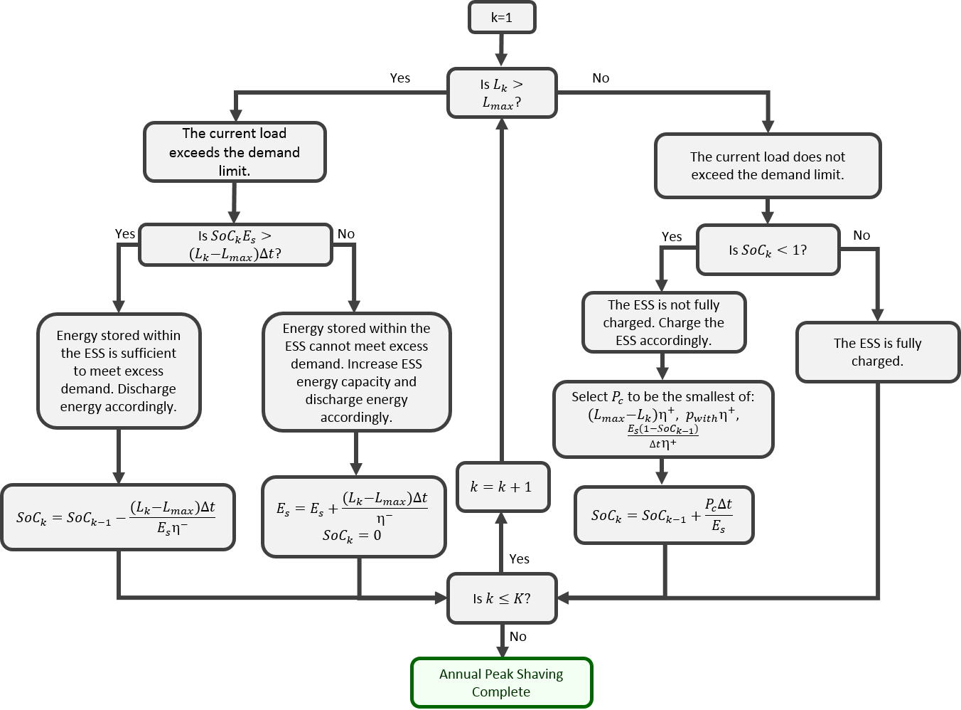
Algorithm
The figure below illustrates the process for determining ESS behavior at each timestep, k, and determining the required ESS energy capacity, \(E_s\).
Variable definitions
\(p_{inj}\): Power injected into the grid by the ESS
\(p_{with}\): Power withdrawn from the grid by the ESS
\(P_{inj,max}\): Maximum ESS injection power
\(P_{with,max}\): Maximum ESS withdrawal power
\(eta^{+}\): Charge efficiency
\(eta^{-}\): Discharge efficiency
\(eta_{rt}\): Round-trip efficiency
\(E_s\): ESS energy capacity
\(SoC\): ESS state of charge
\(SoC_{min}\): Minimum ESS state of charge
\(SoC_{max}\): Maximum ESS state of charge
\(L_{max}\): User-defined demand limit
\(L\): Pre-project load
\(K\): Total number of hours in the optimization period
\(\Delta t\): Elapsed time between steps (here one hour)
Where:
\(p = p_{with} – p_{inj}\)
\(SoC_{k} = SoC_{k-1} + eta^{+} p_{with} – \frac{p_{inj}}{eta^{-}}\)
\(P_{inj,max} = P_{with,max} = max(L_{max} – L_{k})\)
\(eta^{+} = eta^{-} = \sqrt{eta_{rt}}\)
\(0 \leq SoC \leq E_{s}\)